By the end of this guide you will be able to take a folder of documents, convert them into vector embeddings, store those vectors, and answer a natural-language query by ranking documents on semantic similarity rather than exact keyword matches. You will also understand where this approach breaks down, which is often more important than the happy path.
Semantic search rests on one idea: text can be mapped to a point in a high-dimensional space where items with similar meaning land close together. A query like “how do I stop my laptop from overheating” will retrieve a document titled “Preventing thermal throttling in portable computers” even though the two strings share almost no words. That is the appeal. The trouble is that “close together” is defined by a distance metric you choose, a chunking strategy you choose, and an embedding model you choose — and each choice introduces failure modes.
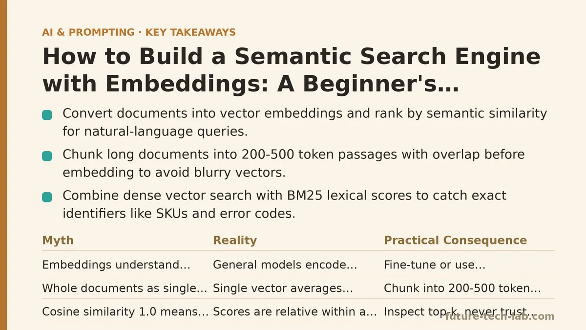
Myth vs. Reality: Five Assumptions Beginners Bring to Semantic Search
Before touching code, it helps to clear out the assumptions that cause most first attempts to underperform. The table below pairs common expectations against what typically happens in a real implementation.
| Myth | Reality | Practical Consequence |
|---|---|---|
| Embeddings understand your domain out of the box | General-purpose models encode general language; niche jargon is compressed toward nearby generic concepts | Fine-tune or use a domain-tuned model when vocabulary is specialized (legal, medical, internal product names) |
| You can embed whole documents as single vectors | A single vector for a long document averages many topics into one blurry point | Chunk documents into 200–500 token passages with overlap before embedding |
| Cosine similarity of 1.0 means “correct answer” | Scores are relative within a query, not absolute; a 0.82 can be the best match in a weak result set | Always inspect the top-k together, never trust a threshold in isolation |
| Any vector database is required from day one | A NumPy array with 10,000 vectors searches in milliseconds | Start with in-memory arrays; adopt a managed vector store only when the corpus or concurrency demands it |
| Semantic search replaces keyword search | Embeddings miss exact identifiers (SKUs, error codes, names) that keywords catch perfectly | Use hybrid retrieval: combine dense vectors with BM25 lexical scores |
The last row is the one that surprises people most. If your users search for “error TS2345” or a specific part number, an embedding model will often dilute that exact token into a fuzzy neighborhood of “TypeScript error” concepts. Lexical search wins there, and no amount of tuning fixes it.
Step 1: Pick an Embedding Model and Understand Its Contract
An embedding model is a function that takes text in and returns a fixed-length vector of floats out. That is the whole interface, but three properties of that contract govern everything downstream.
- Dimensionality. Models commonly output anywhere from 384 to 3072 dimensions. Higher dimensions carry more information but cost more storage and compute per comparison. A 1536-dimension float32 vector is about 6 KB; a million of them is roughly 6 GB before index overhead.
- Max input length. Most models truncate input beyond a token limit (often 512). Text past that limit is silently dropped, which is why chunking matters.
- Training objective. Models trained for symmetric similarity (query-to-query) behave differently from those trained for asymmetric retrieval (short query to long passage). For search, you want an asymmetric retrieval model.
You do not need to train anything to start. A hosted embedding API or an open model running locally is sufficient. The key operational detail is that you must use the same model for indexing and for querying. Mixing models produces meaningless distances because the vector spaces are unrelated.
import os
from openai import OpenAI

client = OpenAI(api_key=os.environ["OPENAI_API_KEY"])

EMBED_MODEL = "text-embedding-3-small"

def embed(texts: list[str]) -> list[list[float]]:
    """Embed a batch of strings. Returns one vector per input string."""
    response = client.embeddings.create(
        model=EMBED_MODEL,
        input=texts,
    )
    return [item.embedding for item in response.data]

# One vector per string, batched to avoid per-call overhead
vectors = embed([
    "Preventing thermal throttling in portable computers",
    "How to cool down an overheating laptop",
])
print(len(vectors), len(vectors[0]))  # e.g. 2 1536
Batching matters. Sending one string per API call multiplies latency and cost by roughly the batch size. Most providers accept dozens to hundreds of inputs per request; check the limit for your provider and stay under it.
Step 2: Chunk Documents Before You Embed Them
Embedding a 40-page PDF as one vector is the single most common beginner mistake. The model has to compress every topic in that document into one point, and the result is an average that matches nothing well. Chunking splits documents into passages small enough to represent one idea.
A workable default is 300 tokens per chunk with 50 tokens of overlap between consecutive chunks. The overlap prevents a sentence that straddles a boundary from being split in a way that loses its meaning in both halves. You tune chunk size against two pressures:
- Smaller chunks give sharper vectors — one topic per vector — but lose surrounding context, so the retrieved passage may be too terse to answer the question.
- Larger chunks preserve context but dilute the vector, and you pay more tokens when you eventually feed the chunk to an LLM.
For most prose documentation, 200–500 tokens is a reasonable starting band. For code or structured records, split on natural boundaries — function definitions or table rows — rather than token count, because a half-function chunk is useless to a reader.
def chunk_text(text: str, chunk_tokens: int = 300, overlap: int = 50) -> list[str]:
    """Split text into overlapping word-based chunks.

    A rough proxy: 1 token is approximately 0.75 words, so multiply
    your token target by 1.33 to get a word target. Replace this with a
    real tokenizer (tiktoken, the model's tokenizer) for precision.
    """
    words = text.split()
    words_per_chunk = int(chunk_tokens * 1.33)
    step = words_per_chunk - int(overlap * 1.33)

    chunks = []
    for start in range(0, len(words), step):
        window = words[start:start + words_per_chunk]
        if window:
            chunks.append(" ".join(window))
        if start + words_per_chunk >= len(words):
            break
    return chunks
The failure mode to watch for: chunks that begin or end mid-sentence and read as nonsense when retrieved alone. Prefer splitting on paragraph or heading boundaries when your source has them, and only fall back to fixed token windows for unstructured text.
Step 3: Store Vectors and Search with Cosine Similarity
A vector store at its core is a table of vectors plus a way to find the nearest ones to a query vector. For a first implementation, a NumPy array is enough. Normalize each vector to unit length, and cosine similarity reduces to a plain dot product, which NumPy computes across the whole corpus in one vectorized operation.
import numpy as np

class InMemoryIndex:
    def __init__(self):
        self.vectors = None      # shape (n_docs, dim)
        self.metadata = []       # parallel list of source info

    def add(self, vectors: list[list[float]], metadata: list[dict]):
        arr = np.array(vectors, dtype=np.float32)
        # Normalize so dot product == cosine similarity
        norms = np.linalg.norm(arr, axis=1, keepdims=True)
        arr = arr / np.clip(norms, 1e-10, None)
        self.vectors = arr if self.vectors is None else np.vstack([self.vectors, arr])
        self.metadata.extend(metadata)

    def search(self, query_vector: list[float], top_k: int = 5) -> list[dict]:
        q = np.array(query_vector, dtype=np.float32)
        q = q / np.clip(np.linalg.norm(q), 1e-10, None)
        scores = self.vectors @ q                      # cosine similarity per doc
        top_idx = np.argsort(-scores)[:top_k]
        return [
            {"score": float(scores[i]), **self.metadata[i]}
            for i in top_idx
        ]

index = InMemoryIndex()
index.add(vectors, [{"id": "doc-1", "source": "thermal.txt"}])
results = index.search(embed(["laptop getting too hot"])[0], top_k=3)
for r in results:
    print(round(r["score"], 4), r["source"])
This exact-index approach is linear in corpus size — every query compares against every vector. With 10,000 vectors of 1536 dimensions, that is about 15 million float multiply-adds, which NumPy finishes in low single-digit milliseconds. At one million vectors it becomes noticeably slower per query, and that is where approximate nearest neighbor indexes (HNSW, IVF) in a dedicated vector database start to earn their place.
When an In-Memory Index Is the Wrong Choice
Do not reach for a managed vector database if any of these hold: your corpus fits comfortably in RAM, your query volume is modest, and you do not need persistence across restarts. Adding one introduces a network hop, an index-maintenance cost, and a new failure surface for a problem a NumPy array already solves. Adopt a vector store when you need filtered search at scale (metadata constraints pushed down into the index), when your vectors exceed available memory, or when multiple services need concurrent access.
Step 4: Verify the Pipeline End to End Before Tuning
Once chunks, vectors, and the index are wired together, the discipline that separates a working system from a flaky one is evaluation on a set of known query-passage pairs. Build a small labeled set: for each query, mark which passages are relevant. Then measure how many of the relevant passages appear in the top-k results.
The two metrics that matter most:
- Recall@k — of all relevant passages, what fraction appear in the top k results. This tells you whether retrieval is finding the answer at all.
- MRR (Mean Reciprocal Rank) — the average of 1/rank of the first relevant result. This tells you whether the right answer is near the top.
A common pattern: recall is fine but MRR is low, meaning the answer is somewhere in the top 10 but rarely in the top 3. That usually points to a ranking problem, not a retrieval problem, and hybrid scoring or a reranker is the fix. Conversely, low recall points to a coverage problem — chunks too large, chunking boundaries splitting answers, or a model that does not encode your domain vocabulary well.
def recall_at_k(index, embed_fn, labeled: list[dict], k: int = 5) -> float:
    """labeled: [{"query": str, "relevant_ids": set[str]}, ...]"""
    hits = 0
    total = 0
    for item in labeled:
        q_vec = embed_fn([item["query"]])[0]
        retrieved = index.search(q_vec, top_k=k)
        retrieved_ids = {r["id"] for r in retrieved}
        hits += len(retrieved_ids & item["relevant_ids"])
        total += len(item["relevant_ids"])
    return hits / total if total else 0.0
Run this before and after every change to chunk size, overlap, or model. Without a labeled set you are guessing, and chunking changes that feel intuitively better frequently make recall worse.
Step 5: Add Hybrid Retrieval When Semantic Search Alone Falls Short
Dense retrieval is strong on paraphrases and weak on exact tokens. Lexical retrieval (BM25) is the mirror image. Combining them covers both. The standard approach is to run both searches, then merge the result lists using Reciprocal Rank Fusion, which combines rankings without needing the two score scales to be comparable.
| Retrieval Method | Strong At | Weak At | Typical Use |
|---|---|---|---|
| Dense (embeddings) | Paraphrase, synonyms, conceptual match | Exact identifiers, rare tokens, codes | Natural-language questions |
| Lexical (BM25/TF-IDF) | Exact strings, names, SKUs, error codes | Wording that differs from the document | Structured lookups, code search |
| Hybrid (RRF merge) | Both of the above | Slightly higher latency and complexity | Production search where queries vary widely |
The RRF formula is simple: for each document, sum 1/(k + rank) across the result lists it appears in, where k is a small constant (commonly 60). Documents ranked highly by either method bubble up.
def reciprocal_rank_fusion(result_lists: list[list[str]], k: int = 60) -> list[tuple[str, float]]:
    """Merge multiple ranked ID lists into one fused ranking."""
    scores: dict[str, float] = {}
    for results in result_lists:
        for rank, doc_id in enumerate(results):
            scores[doc_id] = scores.get(doc_id, 0.0) + 1.0 / (k + rank + 1)
    return sorted(scores.items(), key=lambda x: -x[1])
Where This Approach Falls Apart
Three failure modes recur often enough to plan around them from the start.
Chunk-boundary loss. If an answer spans two chunks and neither chunk contains enough context, the query retrieves neighbors that are each partially relevant and none that answer fully. Overlap mitigates this; so does storing a pointer from each chunk to its parent document and expanding the retrieved chunk with surrounding text before display.
Embedding drift on domain vocabulary. Internal product names, acronyms, and abbreviations get mapped to generic neighbors. A model trained on the public internet has never seen your “payment orchestration service” internal nickname. Options are to add a glossary expansion step before embedding, to fine-tune the model on your corpus, or to lean harder on the lexical half of a hybrid index.
Score thresholds that mislead. Beginners often set a cutoff like “only return results above 0.8 similarity.” Similarity scores are not calibrated across queries — a score of 0.8 on one query is strong and on another is mediocre. Filter on rank (return top-k) rather than absolute score, and if you need a relevance gate, train or calibrate it on your labeled set.
A Practical Build Order
If you are starting today, sequence the work so each step is verifiable before the next:
- Embed a small sample (a few hundred chunks) and manually confirm that clearly related passages score higher than unrelated ones.
- Build the labeled query set — even 30 queries is enough to detect regressions.
- Tune chunk size and overlap against recall@5, not against intuition.
- Add hybrid retrieval only after dense-only recall has plateaued.
- Introduce a vector database only when corpus size, memory, or concurrency forces it.
None of these steps require a large budget or a specialized team. They require a labeled evaluation set and the discipline to change one variable at a time. The most common reason semantic search disappoints is not the embedding model — it is skipping the evaluation step and tuning by feel. Measure first, and most of the decisions downstream make themselves.
🔗 Recommended Reading
- Building Your First RAG Chatbot: A Step-by-Step Tutorial for Beginners
- Function Calling for Beginners: A Step-by-Step Tutorial to Connecting LLMs to External APIs
- Vector Databases Explained: A Beginner's Guide to Storing and Querying Embeddings
- How to Evaluate LLM Outputs: A Beginner's Step-by-Step Tutorial to Testing and Scoring AI Responses
- LLM Guardrails for Beginners: A Step-by-Step Tutorial to Filtering Unsafe Outputs